When it comes to structuring data, many businesses prefer using Google Sheets over Microsoft Excel. If you are one of these people, then you should know that there are extremely useful tricks that you can implement in your work process.

From sending email notifications when something is changed in a table, to creating QR codes, the possibilities within Google Sheets are limitless. Let’s dive further and explore some of the potential uses.

#1 You can add heatmaps to tables

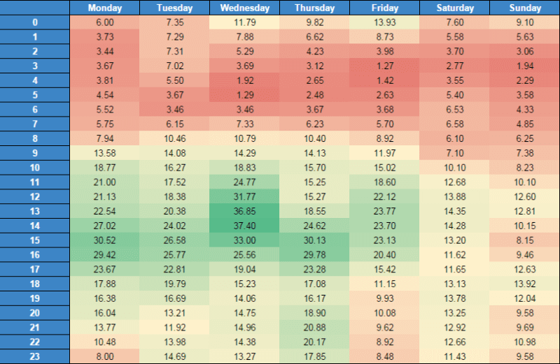
Setting up a heat map in Google Sheets will not only allow you to orientate yourself within a table with just a glance but would also sort things out and make it easier to spot trends. If a particular numerical value is a much-needed threshold for your business or something you want to avoid, then using heatmaps to trigger a colour fill when the target is met can help you recognize the success or failure, without actually having to go through the numbers.

This method can save you a lot of mental energy.

How to do it

Step 1: Select a range of cells with your mouse cursor

Step 2: Right-click, then select “Conditional Formatting” at the bottom.

Step 3: Choose how you would want to format the cells. You can also change the Cell range here, the colour scale, as well as when you want Google Sheets to trigger a colour response.

In order to set it up perfectly, you would want to experiment a bit. But after you’ve done it a couple of times it becomes natural and easy to do.

#2 Protect Cell Data

If you are having trouble with colleagues constantly messing up the data in a certain sheet and you are certain that it isn’t their job to touch it, then you can simply lock the values that shouldn’t be touched by them.

Of course, sometimes there are many different cells and some of them might be part of what your colleagues work on. Thus, you would want to simply lock up the ones that don’t concern them.

This would prevent both conscious and unconscious mistakes.

How to lock the right cells in Google Sheets

Step 1: Select the range of cells you would want to lock. (Or the single cell)

Step 2: Go to view in the top menu bar and select “Protect Range”.

Step 3: Then, go to the protected sheets and ranges panel and select “Add a sheet or range”.

You can also add a description to notify people why these cells are locked and out of their jurisdiction. Moreover, you can simply write a warning to anyone trying to edit the cells, instead of locking them.

#3 Enable Comment Email Notifications

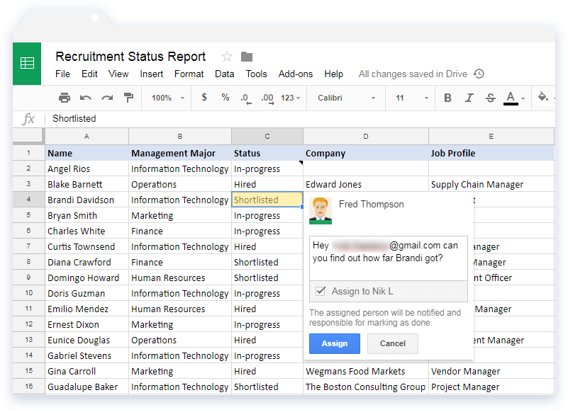
Has it ever happened to you to go through a google sheet and to notice some discrepancy? You want to act right away, without writing things down and fixing them later.
But it isn’t your job or you don’t have the resources or responsibility to fix everything. The best thing is to simply contact the person, responsible for the task.

Instead of calling them, you can simply leave a comment and notify them by email. Since when your computer is online, absolutely everything in Google Drive is updated immediately, they would get an instant notification.

How to notify by email in Google Sheets

Step 1: Leave a comment on the cell that needs the user’s attention and simply add the (+) plus sign, then follow up with either their email address or their name in your contact list.

Step 2: Once you finish the comment, they will get an instant notification by email.

#4 Filters in Google Sheets

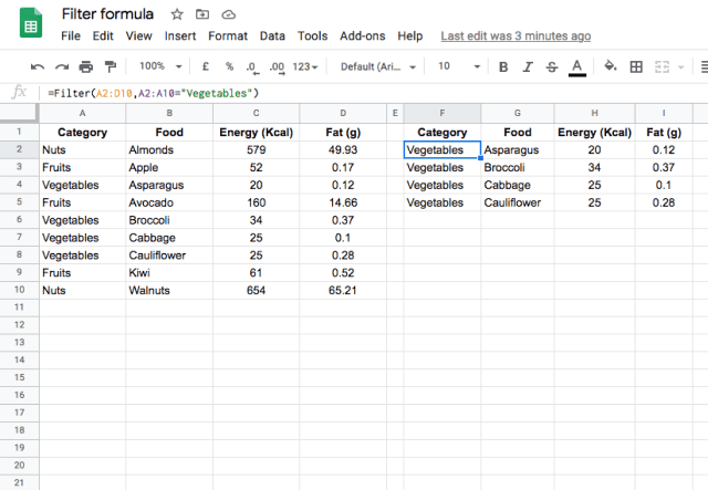
You can create custom filters in Google Sheets. If you are working with much larger databases, then you would need to somehow sort things out. You can even save the filters you create if you need to use them next time by going to “Data” > “Filter Views” > “Create New Filter”, or simply clicking on the filter icon and getting it done through there.

You can filter by:

• Values
• Condition
• Colour
• You can also search through filtered data

How to use filters to sort data

Step 0: Freeze the header, if there is any. (Header rows are rows that contain text and not value and serve for explanation purposes.)

Step 1: Select and highlight the data cells you want to sort.

Step 2: Click on “Data” > “Sort Range”.

Step 3: If you want to make things more organized, write titles for your columns and select the “Data has header row” option.

Step 4: Choose the column you want to sort and select a sorting order, then simply click “Sort”.

You can also always add more sort columns if needed.

#5 You can import an RSS feed or website data straight into Google Sheets

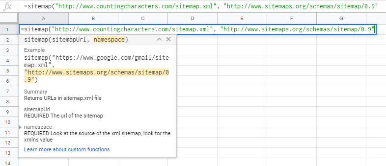
You can import data from a website or an RSS feed in order to make a products table, a sitemap, among other things. The primary data sources that you can use for that are feeds like:

• ImportXML feed, which can allow you to identify a custom section within a certain web page.
• An ImportFeed, which serves the purpose to import RSS entries.
• ImportHTML, which can be used to set up tables and lists via HTML
• ImportData, which is primarily used to add CSV files to sheets.

#6 You Can Validate Google Sheets Cell Data

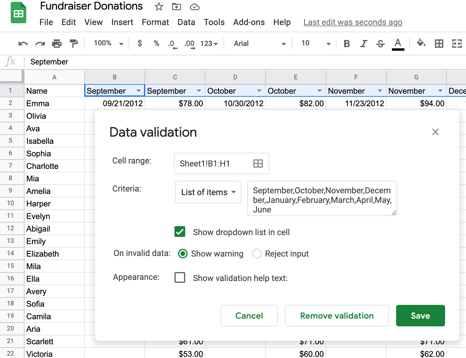
Data validation certainly matters since you can sometimes type in input errors like placing dates where there should be numbers, or putting random text where there should be prices.

For example, when you are assessing tests of colleagues or school exams, you need to have a maximum number of points the examination subject can score.  Thus, you would want to place an upper limit for the cells which reflect the test score.

Data validation within google sheet cells can also be used to minimise the number of misspellings and unwanted values input. You can even make it possible for the user to eliminate typing altogether by implementing drop-down lists.

Such can be used when selecting months, time periods, grades, quality, and many more.

If you are selling green, red, and yellow apples, you would want the cell to include only these three symbols for sorting purposes (G for green, R for red and Y for yellow.)

How to validate google sheets cell data

Step 1: Select a range of cells, then go to Data validation.

Step 2: In the filled form, check the selection of cells, then proceed to criteria and type in the G, R, Y (in our case). Tick “Show dropdown list in cell”.

Step 3: The next thing you have to do is to select show warning or reject input on invalid data. (This entirely depends on your choice.)

And this is it. You’ve successfully limited the things that can be written down in a certain cell within your google sheets document.

#7 How to remove unprintable characters with Google Sheets

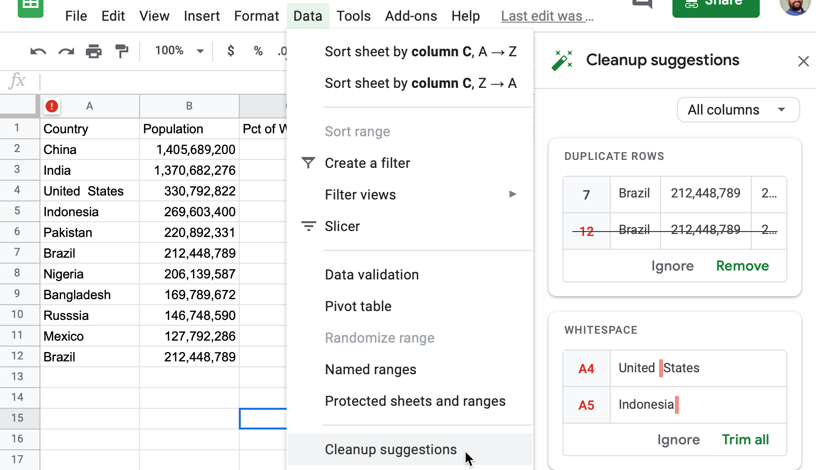
Sometimes, there are typos, duplicates, unnecessary text or intervals. Although these are hard to find, when someone does find them, it makes the entire table feel unprofessional.

Even worse, it makes you think whether there are some major inconsistencies throughout the data. If someone is careless enough to commit lexical errors, what about the data?

You can easily clean this by using cleanup suggestions.

Another useful trick is to check whether there are any non-printable characters within your sheet before printing or presenting it. You can do that by selecting the cell, right-clicking and using the Clean and Trim functions, which can remove the whitespace in the end and the start of the cells, before the text.

#8 Use Google Sheets to Translate Text

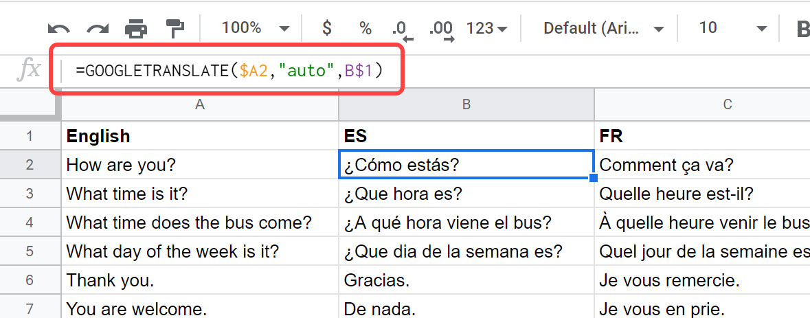
Although this isn’t a main function of sheets, Google always tends to integrate their products with one another. There is actually a function that can be written within the cells to translate text.

That can be useful if you are making a dictionary, a glossary, or you have a large list of terms you need to be translated so that your foreign employees can understand them better.

You can do that for as many languages as you want, as long as they are supported by Google Translate.

#9 How to use Automatic Capitalization in Google Sheets

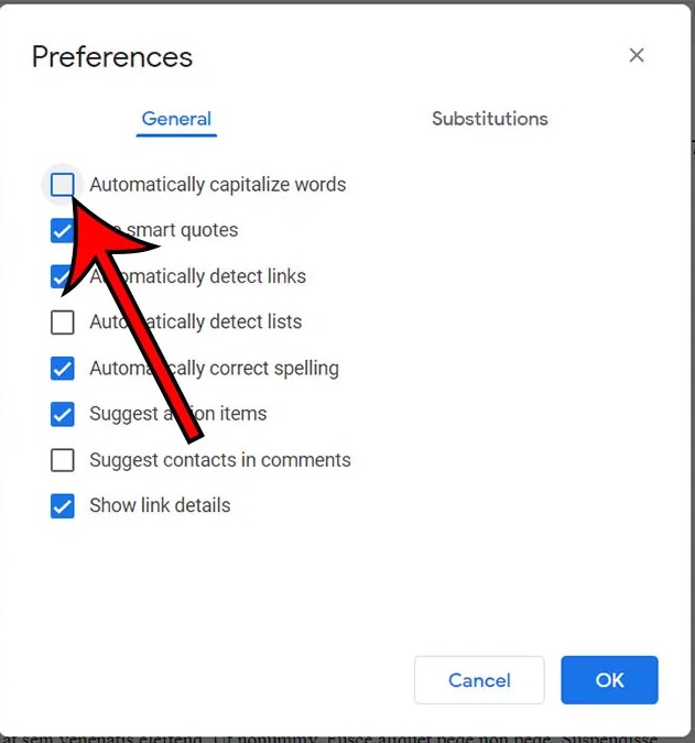
If you are making a database full of names of cities, people, companies, countries or anything else that needs capitalization, instead of typing everything yourself and smashing down that shift or caps lock key, you can easily turn on this function and save some time and effort.

In order to do so:

Step 1: Go to “Tools”.

Step 2: Select the “Preferences” Tab.

Step 3: Like in the image above “Check the AUtomatically capitalize words box.

If you are struggling with the opposite, and Google Sheets is capitalising your words for no reason, you can simply uncheck the box or use the “LOWER” function to make all letters minuscule.

#10 Use Google Sheets to check the validity of an Email address

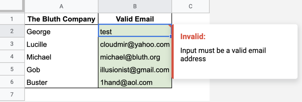
Let’s say you have a list of emails to use and run through a group to send a message with the help of outlook or some other free email service, which doesn’t have the qualities of a professional CRM system.

If you have a ton of wrong emails, lacking symbols or including invalid letters, you would get a bunch of errors, slowing you down.

If you want to eliminate the wrong email address syntaxis, then simply use the ISEMAIL function within google sheets, which allows Google to check whether the email is properly written. It will immediately highlight the emails that are missing a “.com” or a “@” part of the traditional email address structure.

Other similar functions of Google sheets are to check whether a URL link is working. This can be done with the help of the ISURL function. You can read more about both functions and how to use them – Here.

#11 Use A Sparhline Graph to Visualize Data Points Within Google Sheets

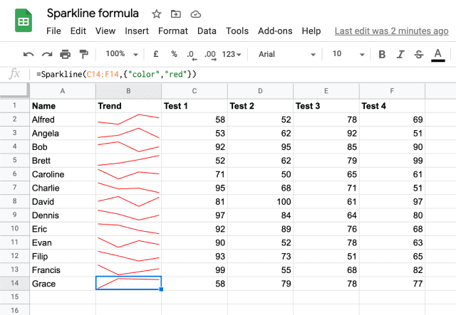
Sometimes numbers get confusing. If you have 30 periods of time that you have to compare, it gets difficult to follow the trend throughout each data point.

Luckily, a sparkling can easily depict the movement of each variable across time. You can implement individual graphs for the progress or regress of each variable, and compare the results.

Some products or people start with very slow progress, but eventually grow higher and higher, while others have a better start but lag behind later on. Spotting similar trends can help you allocate resources better, regardless of whether you are managing products, services, or people.

The name of the function to use here is SPARKLINE, and you can place it anywhere, and select its colour.

#12 Google Sheets can generate QR Codes

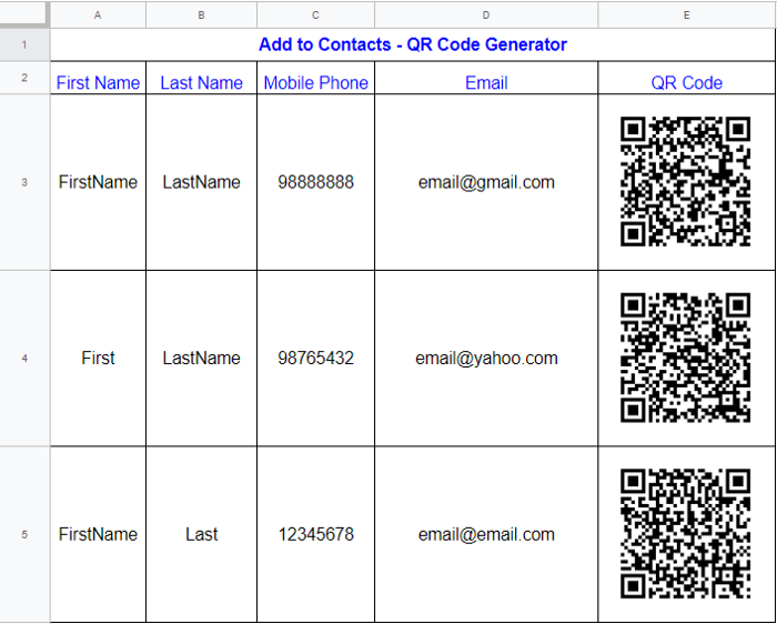
Believe it or not, you don’t need to install some expensive fancy software in order to generate QR codes for your business. Google Sheets can do the trick for you.

These can be used for product storage, tracking people attending an event, a conference, a group meeting, or you can even place them on a poster somewhere for promotional purposes.

In order to generate a QR code via Google Sheets, you would need to place several pieces of information in one or more cells in google sheets, and let the system use it to generate a personalized QR code, based on that information alone.

You can read more on how to use the function properly, and learn more about the uses of QR codes – Here.

#13 Learn the Basic Formulas

At first, exploring Google Sheet Formulas seems like a nightmare, but once you know what you’re doing, it actually speeds up any process a ton.

If you want to know more about a certain function, instead of taking the time to google it, you can simply write it in the google sheets function tab and once you place a parenthesis, hover over it with your cursor.

That would make an explanatory field of text pop up and tell you all you need to know about the given function. It will share with you the types of valuable points that you need to insert “Numbers, text, Dates, etc.”, as well as how to start or end the function.

Conclusion

There are thousands, if not millions of uses for Google Sheets. Whether you are using it for accounting, for building databases, or simply for storing some useful information, you can facilitate the process by learning a few formulas and functions.

Knowing the possibilities of the platform can further inspire ideas into your work. As seen above in the article, you can use Google Sheets as a communication platform between teams by assigning tasks. You can create charts, import data, group up, filter and sort anything. The possibilities are endless. Go ahead and explore.